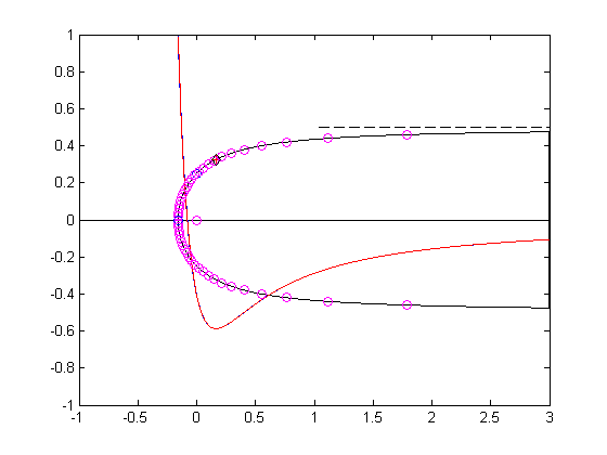
The Rankine nose or Rankine leading edge is an example of flow around the leading edge of a symmetric aerodynamic body which is symmetric about the x-axis of coordinate system.This flow can be obtained by adding a uniform flow and a source flow at the origin.The velocity potential and stream function of this flow is

\[\phi=U_{\infty}x+\frac{m}{4\pi}ln\left ( x^{2}+y^{2} \right )\;,\;\psi=U_{\infty}y+\frac{m}{2\pi}tan^{-1}\frac{y}{x}\]

The velocity field for this flow is \[u=U_{\infty}+\frac{m}{2\pi}\frac{x}{x^{2}+y^{2}}\;;\;v=\frac{m}{2\pi}\frac{y}{x^{2}+y^{2}}\]

Matlab solution to the problem is

clear;clc
disp('Example: Rankine nose')
m = 1; % Source strength for source at (x,y) = (0,0).
V = 1; % Free stream velocity in the x-direction
disp(' V m ')
disp([V m])
disp(' Velocity potential:')
disp(' phi = V*x + (m/4/pi)*log(xˆ2+yˆ2)')
disp('Stream function:')
disp(' psi = V*y + (m/2/pi)*atan2(y,x)')
disp('The (x,y) components of velocity (u,v):')
disp(' u = V + m/2/pi * xc/(xˆ2+yˆ2)')
disp(' v = m/2/pi * y/(xˆ2+yˆ2)')
%
xstg = - m/2/pi/V; ystg = 0; % Location of stagnation point.
%
N = 1000;
xinf = 3;
xd = xstg:xinf/N:xinf;
for n = 1:length(xd)
if n==1
yd(1) = 0;
else
yd(n) = m/2/V;
for it = 1:2000
yd(n) = (m/2/V)*( 1 - 1/pi*atan2(yd(n),xd(n)) );
end
end
end
xL(1) = xd(end); yL = -yd(end);
for nn = 2:length(xd)-1
xL(nn) = xd(end-nn); yL(nn) = -yd(end-nn);end
plot([xd xL],[yd yL],'k',[-1 3],[0 0],'k'),axis([-1 3 -1 1])
u = V + m/2/pi * xd./(xd.^2+yd.^2);
v = m/2/pi * yd./(xd.^2+yd.^2);
Cp = 1 - (u.^2+v.^2)/V^2;
hold on
plot(xd,Cp),axis([-1 3 -1 1])
plot(0,m/V/4,'o')
plot(xstg,ystg,'o')
plot([1 3],[m/2/V m/2/V],'--k')
[Cpmin, ixd] = min(Cp);
xmin = xd(ixd);
ymin = yd(ixd);
plot(xmin,ymin,'+r')
Cpmin;
% Computation of normal and tangential velocity on (xd,yd):
phi = V*xd + (m/4/pi).*log(xd.^2+yd.^2);
dx = diff(xd); dy = diff(yd); ds = sqrt(dx.^2 + dy.^2);
dph = diff(phi); ut = dph./ds; xm = xd(1:end-1) + dx/2;
psi = V*yd + (m/2/pi).*atan2(yd,xd);
plot(xm,1-ut.^2/V^2,'r')
%
% Check on shape equation
%
th = 0:pi/25:2*pi;
r = (m/2/pi/V)*(pi - th)./sin(th);
xb = r.*cos(th);
yb = r.*sin(th);
plot(xb,yb,'om')
%
% Exact location of minimum pressure
thm = 0;
for nit = 1:1000
thm = atan2(pi-thm,pi-thm-1);
end
thdegrees = thm*180/pi;
rm = (m/2/pi/V)*(pi - thm)/sin(thm);
xm = rm*cos(thm);
ym = rm*sin(thm);
plot(xm,ym,'dk')
um = V + m/2/pi * xmin/(xmin^2+ymin^2);
vm = m/2/pi * ymin/(xmin^2+ymin^2);
Cpm = 1 - (um^2+vm^2)/V^2;

Rankine nose solution